VLOOKUP Hack #1: Sort Order
VLOOKUP is one of the most popular Excel functions. It can do amazing things and help save time. But, there are some really cool hacks that make it even better. This is the first post in a series of VLOOKUP Hacks.
Hope you enjoy 🙂
Issue
VLOOKUP Hack #1 helps address the sort issue. Sort issue? Yes, and the sort issue has confuzzled many an Excel user over the years.
I’ve included a short video demonstration as well as a detailed narrative below for reference.
Video Demonstration
https://youtu.be/HqXgkrEVwBU
Detailed Narrative
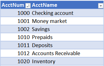
Let’s say we wanted to use VLOOKUP to retrieve an account name based on the account number from a chart of accounts, as shown below.
Assuming the lookup value is B7, the lookup range is Table1, and the account name is in the second column, we could use something like this in C7:
Assuming the lookup value is B7, the lookup range is Table1, and the account name is in the second column, we could use something like this in C7:
=VLOOKUP(B7,Table1,2)
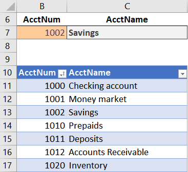
When the table is sorted in ascending order by the lookup column, the AcctNum column, you get the expected result. For example, if the AcctNum is 1002, the VLOOKUP function above returns the expected account name, Savings, as shown in C7 below.
But, if the table get sorted by AcctName instead, we get an unexpected result, as shown below.
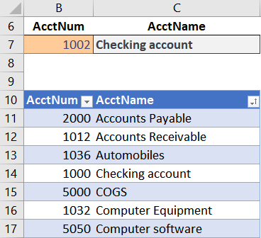
Wait, what? 1002 is not Checking account, yet, that is what VLOOKUP returns … is it broken? Is the formula wrong? What’s up? Do I have to sort by the lookup column? What is going on here?
These questions all bring us to our first hack.
Hack
So, the VLOOKUP formula above is written like this:
=VLOOKUP(B7,Table1,2)
You will notice that 3 arguments are defined, B7, Table1, and 2.
But, here is the hack: there is an optional 4th argument!
When the 4th argument is omitted, as in the formula above, it takes on a default value. So, we need to unpack this mysterious 4th argument to understand what is happening.
The 4th argument controls the behavior of VLOOKUP in a couple of key ways, including, as you may suspect, the sorting requirement. Officially, the 4th argument is called the range_lookup argument. Practically, it tells Excel whether you are looking for an exact matching value, or, a value between a range of values. It is a Boolean argument, so it expects a TRUE or FALSE value. (Alternatively, you can use 0 instead of FALSE and any non-zero number instead of TRUE.) TRUE means you are looking for a value between a range of values, and FALSE means you are looking for an exact matching value. I’ll expand this idea more in the next post, but for now, I want to stay focused on the sort issue.
When the 4th argument is TRUE, the data must be sorted in ascending order to return an accurate result. However, when the 4th argument is FALSE, the data need not be sorted…any order is fine.
So, when the 4th argument is TRUE, you may get an unexpected result if the data is not sorted in ascending order by the first column in the range. And, that is exactly what we saw above. We got an unexpected result. Instead of 1002 returning Savings, it returned Checking account. But, if we inspect the formula, we can see that we did not specify TRUE or FALSE for the 4th argument. We simply omitted it.
Here is the key: when omitted, the 4th argument is TRUE.
That means that when we write a VLOOKUP, and don’t specify the 4th argument, it defaults to TRUE. That means, sort order matters! When the data is not sorted in ascending order by the first column, you may get unexpected results.
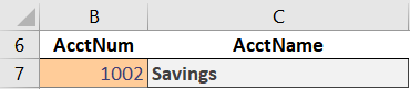
So, we can resolve the issue by using FALSE (or 0) as the 4th argument, as shown below.
=VLOOKUP(B7,Table1,2,FALSE)
With that update to our formula, it returns Savings, as expected:
So, remember this: when the 4th argument is TRUE or omitted, the lookup range must be sorted in ascending order by the first (lookup) column to return an accurate result. But, when the 4th argument is FALSE (or 0), the data does not need to be sorted.
In the next post, we’ll examine the 4th argument in more detail. It allows us to perform some really fun lookups!
- Sample Excel File👇👇👇👇👇

Comments
Post a Comment